Excel Shortcuts - An Overview

By pushing ctrl+shift+center, this will determine as well as return worth from numerous varieties, as opposed to just individual cells included to or increased by each other. Determining the sum, item, or ratio of private cells is very easy-- just use the =AMOUNT formula as well as enter the cells, values, or array of cells you desire to perform that arithmetic on.

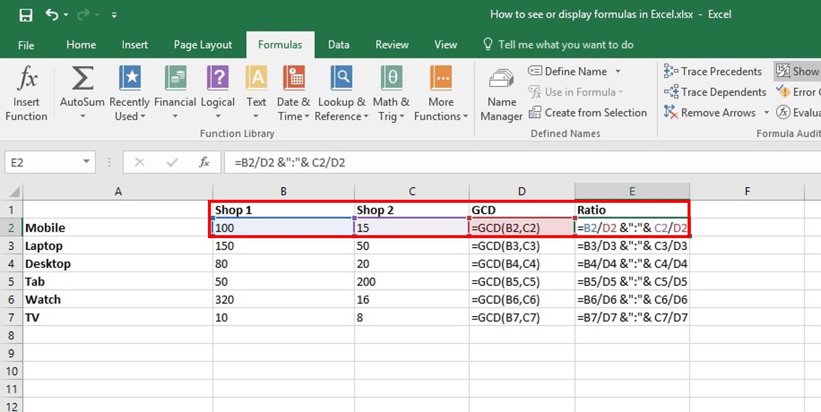
If you're looking to find overall sales earnings from a number of marketed devices, as an example, the selection formula in Excel is perfect for you. Below's just how you 'd do it: To begin utilizing the array formula, kind "=SUM," and in parentheses, enter the initial of two (or three, or 4) ranges of cells you would love to multiply with each other.

This represents reproduction. Following this asterisk, enter your 2nd range of cells. You'll be multiplying this second series of cells by the first. Your development in this formula should currently appear like this: =AMOUNT(C 2: C 5 * D 2:D 5) Ready to press Enter? Not so fast ... Due to the fact that this formula is so complicated, Excel reserves a various keyboard command for varieties.

This will certainly acknowledge your formula as a variety, wrapping your formula in brace personalities and also efficiently returning your item of both varieties combined. In revenue estimations, this can lower your time and effort considerably. See the final formula in the screenshot over. The MATTER formula in Excel is denoted =MATTER(Beginning Cell: End Cell).

For example, if there are 8 cells with gone into values in between A 1 and also A 10, =COUNT(A 1: A 10) will certainly return a value of 8. The MATTER formula in Excel is especially valuable for huge spreadsheets, in which you intend to see the amount of cells contain actual entries. Don't be misleaded: This formula will not do any kind of math on the worths of the cells themselves.

6 Easy Facts About Excel Shortcuts Shown

Making use of the formula in strong above, you can easily run a count of active cells in your spreadsheet. The result will look a little something like this: To do the ordinary formula in Excel, go into the worths, cells, or variety of cells of which you're determining the average in the format, =AVERAGE(number 1, number 2, etc.) or =AVERAGE(Beginning Worth: End Value).

Discovering the standard of a range of cells in Excel keeps you from having to locate private sums and then carrying out a separate department formula on your total. Using =AVERAGE as your preliminary text entry, you can let Excel do all the work for you. For referral, the average of a team of numbers amounts to the sum of those numbers, divided by the variety of things in that team.

This will certainly return the sum of the worths within a preferred variety of cells that all meet one requirement. For example, =SUMIF(C 3: C 12,"> 70,000") would certainly return the amount of values in between cells C 3 as well as C 12 from just the cells that are greater than 70,000. Let's claim you wish to establish the revenue you created from a checklist of leads that are associated with specific area codes, or compute the amount of particular employees' salaries-- however only if they fall over a particular amount.

With the SUMIF function, it does not have to be-- you can easily accumulate the amount of cells that satisfy specific requirements, like in the salary instance over. The formula: =SUMIF(array, requirements, [sum_range] Variety: The array that is being checked utilizing your criteria. Requirements: The criteria that determine which cells in Criteria_range 1 will be combined [Sum_range]: An optional series of cells you're going to accumulate along with the initial Range got in.

In the instance below, we wished to compute the sum of the salaries that were higher than $70,000. The SUMIF function built up the dollar quantities that surpassed that number in the cells C 3 with C 12, with the formula =SUMIF(C 3: C 12,"> 70,000"). The TRIM formula in Excel is represented =TRIM(text).

The Ultimate Guide To Excel Skills

For instance, if A 2 consists of the name" Steve Peterson" with undesirable rooms before the given name, =TRIM(A 2) would return "Steve Peterson" without rooms in a brand-new cell. Email and file sharing are terrific tools in today's office. That is, till among your associates sends you a worksheet with some truly funky spacing.

Instead of painstakingly eliminating and also adding rooms as required, you can tidy up any uneven spacing using the TRIM function, which is made use of to get rid of additional areas from information (with the exception of solitary spaces in between words). The formula: =TRIM(message). Text: The message or cell from which you want to get rid of rooms.

To do so, we went into =TRIM("A 2") into the Solution Bar, and replicated this for every name below it in a new column alongside the column with unwanted areas. Below are some various other Excel formulas you could locate helpful as your information monitoring needs expand. Allow's claim you have a line of text within a cell that you intend to break down right into a few various sectors.

Function: Used to remove the initial X numbers or characters in a cell. The formula: =LEFT(text, number_of_characters) Text: The string that you desire to remove from. Number_of_characters: The variety of characters that you wish to remove beginning from the left-most character. In the instance below, we went into =LEFT(A 2,4) into cell B 2, and replicated it right into B 3: B 6.

Function: Utilized to extract characters or numbers between based upon position. The formula: =MID(text, start_position, number_of_characters) Text: The string that you desire to remove from. Start_position: The position in the string that you wish to start extracting from. For instance, the initial placement in the string is 1.

Excel Jobs Can Be Fun For Anyone

In this example, we got in =MID(A 2,5,2) into cell B 2, as well as copied it into B 3: B 6. That allowed us to extract both numbers starting in the 5th setting of the code. Objective: Used to draw out the last X numbers or characters in a cell. The formula: =RIGHT(message, number_of_characters) Text: The string that you desire to extract from.

formula excel weekend excel formulas index match formula excel greater than